Judith I. Stallman
Professor emeritus agricultural and applied economics and public affairs

Austin Sanders
Master’s student in agricultural and applied economics

During the past recession (2008–2009) and in its aftermath, local governments struggled to manage budgets as revenues fell. Experienced officials had managed through a past economic cycle and, as a result, many local governments had larger reserve funds than in the past for managing through these cycles. However, the past recession was deeper and longer than any in the past half-century with a slower recovery, and these funds were not sufficient. With lower revenue, the majority of local governments struggled to meet the needs and expectations of citizens and experienced fiscal stress.

With the current pandemic, the economic downturn was swifter than the past recession and local governments again face budget difficulties. The data do not cover the current pandemic. In addition, at any time short-term factors and unpredictable events, such as snowstorms, flooding and drought, can cause both increased demand for government services by the residents while at the same time lowering tax revenues.

After the Great Recession of 2008–2009, local governments’ budgets did not recover at the same pace as the economy. Longer-term trends, which develop slowly and might not immediately come to the attention of local officials, may have been the cause of the slow recovery. These trends include economic changes, which the existing tax structures do not take into account (White, 2017), demographic changes, and more cautious businesses and consumers as a result of the recession. In addition, new laws, rules and mandates from the state government, or local government decisions, such as taxes and tax incentives, may affect the recovery of local budgets (White, 2017).

An example of an economic change is how consumer spending is changing. Many state and local governments rely on sales tax revenues for an important part of the budget. E-commerce has had an impact on sales tax revenues, and is an example of the tax system being out of step with the economy. But there are additional factors that affect sales tax revenues. Because of low inflation and slowing demand, retail prices remain low. As a result, sales tax revenues, which are a percentage of price, will not grow as fast as the economy (White, 2017). An often overlooked factor is that the service sector is the fastest growing part of the economy. Consumers are allocating an increasing share of their spending to services, which are not broadly taxed, and decreasing the share of their spending on retail goods (Bureau of Economic Analysis). This is another example of an economic trend the tax system, based on an older economy in which goods are taxed but most services are not, does not capture.

A further example of a long-term trend affecting local governments is population change. In Missouri, many rural areas are losing population. Public finance theory outlines the implications for governments with different patterns of population growth. Counties have a set of fixed costs they must meet — for example, the courthouse, courts, recorder, elections and bridge repair. Jurisdictions losing population must still provide and maintain basic infrastructure and services. That means these costs must be spread across a smaller population, resulting in higher costs per capita. Falling or slow population growth may lead to lower property values and taxable sales if there is not sufficient demand to keep businesses open. This pattern likely leads to fiscal stress (Sanders and Stallmann, 2019).

Jurisdictions with fast population growth have more population over which to spread fixed costs so that average costs may be lower. Economists call this “economies of scale.” In addition, population growth may increase property values and the sales tax base. On the other hand, population growth means that, at some point, the jurisdiction will outgrow the capacity of its infrastructure and services. Increasing capacity, especially of physical infrastructure, will require increased expenditures and may cause fiscal stress, at least in the short run.

Fiscal ratios: Indicators of fiscal conditions

Local governments need a way to evaluate their financial condition over time in order to pinpoint the sources of fiscal stress — are they short run, such as a natural disaster, or are they part of longer-term trends? Businesses monitor their financial condition using a set of financial ratios. A similar approach can be useful for governments. This report contains a set of fiscal ratios calculated from the budgets of Missouri’s third class counties because no single ratio can reflect the complexity of local governments. Trends for these ratios from 1996–2013 can provide information on both short- and long-run economic trends (Maher and Nollenberger, 2009).

Gorina and Maher (2016) defined fiscal stress as follows: when a city took any one of 14 budget actions, such as laying off or furloughing employees or delaying payments to vendors or pensions. They began with 48 fiscal ratios recommended by the International City Managers Association and a set of demographic and economic factors. Similar to how bond ratings agencies develop their ratings, they used a model with cities in several states to test which aspects of demography, economy and the budget were most important in mitigating or contributing to fiscal stress from 2007 to 2012. They found that decreasing cash balances as a percentage of expenditures increased fiscal stress. They also found that a higher percentage of revenues from the property tax decreased fiscal stress. In addition, fiscal stress was higher from 2008 to 2012 than in 2007. This indicates that economic factors beyond the control of cities slowed recovery and affected their fiscal standing.

The objectives of this report are to:

• document various patterns of population change in third class counties from 1996 to 2017,
• examine the impact of population change on selected fiscal ratios,
• examine the direction of trends for fiscal ratios by population change, and
• examine whether volatility is associated with population change.

Data and analysis

Among the many services counties provide are roads and bridges, law enforcement, courts, elections, recording of deeds, and tax collection. It is expected that a county with a large population will have larger tax bases and a larger budget than one with a smaller population. It might also be expected that wealthier counties will have larger tax bases and budgets than counties with fewer resources. One way to compare counties with different populations, tax bases and budgets is to compare fiscal ratios rather than budget totals. Trends in the various fiscal ratios by patterns of county population change may provide insights into how population trends affect county budgets.

Missouri’s county classification

Missouri has 114 counties and one independent city, St. Louis City. By the constitution, counties are classified into four classes based on their assessed valuation (Missouri Association of Counties, 2017). This report focuses on third class counties. A third class county has assessed property value of less than $600 million (Missouri Association of Counties, 2017). Currently, the Missouri Secretary of State classifies 89 counties as third class (Secretary of State, 2016).

While the data are specific to the third class counties, they may be useful to other governmental jurisdictions within a county. Counties, cities, school districts and special districts have different spending priorities, but they share the population and draw on the same tax bases.

Patterns of population change

This report divides the third class counties into four categories based on their population change from 1996 to 2017, the years for which we have budget data.

Population-loss counties declined in population from 1996 and 2017. Their population-loss rates range from a negative 24.1% to 0.0%. The 31 counties in this group are mainly north of the Missouri River, but there are some in the Bootheel region and in the Ozarks (Figure 1).

Slow-population-growth counties grew less than the average population growth rate of third class counties (3.7%). Their population growth rates range from 0.0% to 2.9%. There are 17 counties in this group.

Medium-population-growth counties grew between the third class average growth rate (3.7%) and Missouri’s population growth rate (12.6%). There are 24 counties in this group, and population growth rates range from 4.5% to 12.5%.

High-population-growth counties grew more rapidly than the state of Missouri. Their population growth rates range from 13% to 23.3%. There are 14 counties in this group. Most of these counties are south of the Missouri River, near urban areas and in tourism areas. Near urban areas, families may be locating for jobs that are in that county or in neighboring counties.

Pulaski, Warren and Webster are third class counties but are excluded from this report for several reasons. First, they are in a category by themselves in terms of population growth (38%, 55% and 38% respectively). Second, three observations will not provide statistically reliable averages, and some of the fiscal data for these counties are missing. In addition, Pulaski County is heavily influenced by U.S. military policy and is not representative of any other county in Missouri.

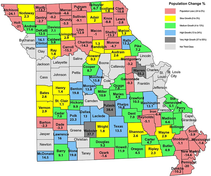
Figure 1. Third class counties by population change: 1996–2017.

Information about the budgets

The revenues and expenditures for this report are from the annual budgets that third class counties submit to the state. Annual county budget documents contain three years of data: actual data for the past year, data for the current year, which is a mix of actual data and projections for the rest of the year, and the projected budget for the next year. The most recent data are from the budget document for 2017. In examining the fiscal trends in the following graphs, it is important to remember that the data for 2016 and 2017 are not the final budget numbers for those years, and 2015 is the most recent final budget data.

From 2005 onward, the data are not audited and may contain errors. It is unlikely that an error in a single county will have a large impact on the average for a group of counties. In addition, counties report their budgets in several formats so that we do not have data on every third class county for every year. For each year, we calculate the trends in the fiscal ratios using only the counties for which there are standard budgets for that year.

The report focuses on tax bases and revenues rather than expenditures because these two items more accurately reflect the fiscal conditions. That is, counties must work within the constraints of their tax bases and the revenues they provide at the beginning of the fiscal year. Expenditures must be adjusted to fit revenues. While revenues can be increased by adjusting tax rates, this adjustment cannot happen until the next fiscal year.

The ratios presented below do not include debt. As a result, the ratios focus on short-term budget trends and how they compare across county population growth types.

General fund fiscal ratios

As population changes, counties’ per capita costs of providing services change in two ways. First, economies of scale exist when an increase in production results in a decrease in the per unit cost of production. A similar idea for counties is the per unit cost of a service, which can be thought of as the cost per citizen or per capita cost. Counties with growing populations may find that the per capita cost for a service decreases as they increase the total amount of the service to provide it to more citizens. However, counties with small populations have limited ability to lower per capita costs. For population-loss counties, the government may not be able to cut all services in direct proportion to the fall in population. If they lose population and produce a lower total amount of a service, the per capita cost of providing that service may increase. Second, for some services, such as roads, counties may need to continue to produce the same level of services, but if that cost is spread among fewer people, the per capita cost per mile increases. These can be thought of as fixed costs and when spread over fewer people, require higher revenues per capita.

If population is growing, the county may be able to provide services to more people at a lower cost per person. At the same time, rapid population growth may create capacity constraints that require large investments to accommodate the growing population. For example, there may be increasing congestion on a bridge, creating a need for additional lanes. Generally, when such improvements are made, additional capacity is constructed to accommodate future growth. The initial investment may increase the per capita cost of services. However, once the initial investment is made, the per capita bond repayment and operational costs decrease as population grows.

For counties, revenues are closely related to expenditures or costs, as budgets must be adjusted to fit the revenues available in any given budget year. General fund own-source revenues are the revenues a county generates from its own sources of revenue and can adjust upward or downward. Counties also receive revenues from other sources, such as the state or federal government or through contracts with other local governments. Increasing revenues per capita generally reflect increasing costs or expenditures per capita, an indicator of fiscal stress. In addition to increasing costs per capita, necessitating increasing revenue, revenues per capita may increase to meet an increase in residents’ demand for more services from the county or increasing costs due to inflation. To control for the need to increase revenues because of inflation, Figures 2a and 2b display the current dollar values as well as inflation-adjusted dollars. The Municipal Cost Index (Penton Media Inc., 2018) is used to adjust for inflation.

General fund revenues per capita

Revenues in the general fund can be used to fund any goods or services the county provides. Only the general revenues under direct control of county government (own source revenues) — taxes, fees and charges, and miscellaneous revenues — are included in Figures 2a and 2b. Counties can adjust own-source revenues to respond to changing fiscal conditions. Miscellaneous revenues include the sale of used equipment, grants for various purposes, reimbursements, etc. Intergovernmental revenues are another source of  funds. Counties have less control over these (see page 8).

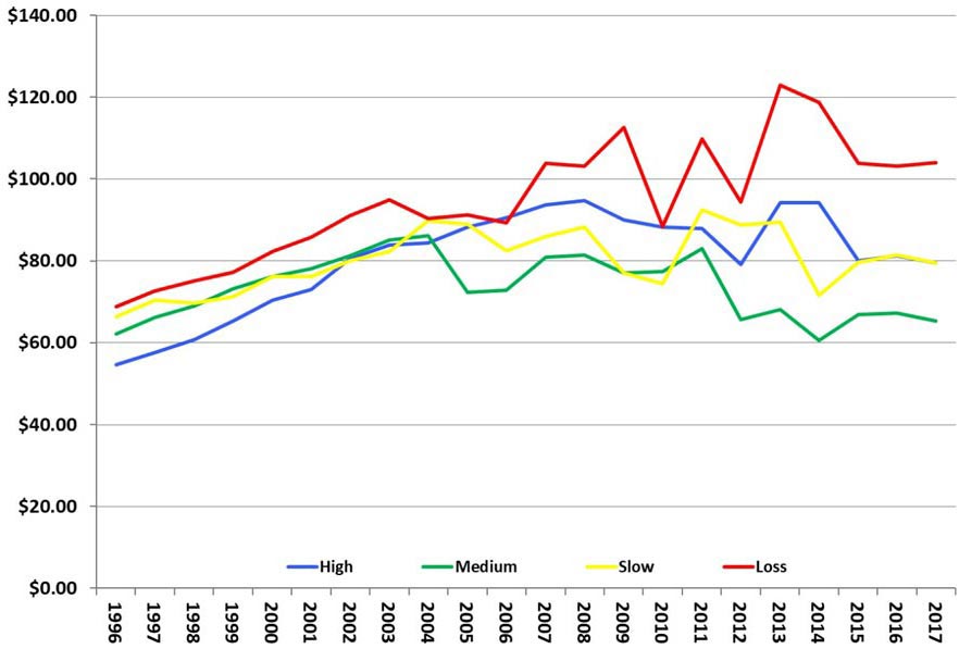
Figure 2a. General fund tax revenues + fees and charges + miscellaneous revenues per capita.

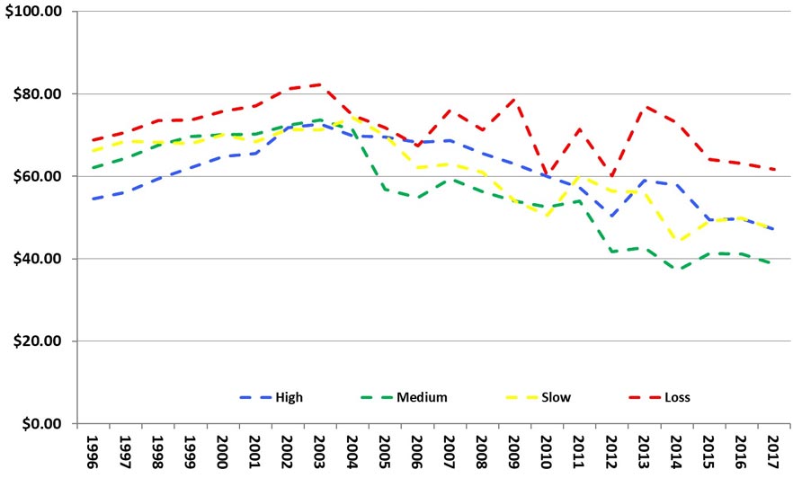
Figure 2b. General fund tax revenues + fees and charges + miscellaneous revenues per capita: adjusted for inflation.

All county types had increasing general fund own-source revenues per capita from 1996 to 2003 (2004 for the slow-growth counties), even with inflation-adjusted dollars. From that point onward, all counties have declining inflation-adjusted revenues. For all counties, inflation-adjusted own-source revenues are lower at the end of the period than in 1996. For the medium- and slow-growth counties, the decline is 33% and 25%, respectively. For high-growth and population-loss counties, the declines are 10% and 7% respectively. Total revenues and revenues per capita may be expected to decline in the short run during a recession, because tax bases may decline. During the recovery they would be expected to return to pre-recession levels. Declining own-source revenues per capita in the post-recession period are an indication that fiscal stress is declining.

In addition, the inflation-adjusted own-source revenues show volatility. It is most pronounced for the population-loss counties; volatility begins with the recession. For the slow-growth counties, though, volatility begins with the recovery. Volatility can be an additional source of fiscal stress as it makes planning difficult.

Comparing county types shows that population-loss counties have the highest revenues per capita. Given that this is consistent throughout the period, it is an indicator of higher per capita costs, which may lead to fiscal stress. High-population-growth counties began the period with the lowest own-source revenues per capita. Since the recession, they have the second highest revenues per capita. This suggests they may be facing capacity constraints and the need to increase revenues, an indicator of fiscal stress.

General fund revenues per $100s of income

Of counties’ own-source revenues, taxes, and fees and charges are paid from residents’ income. Revenues per $100 of county personal income measures counties’ tax efforts. An increasing tax effort over time is an indicator of potential fiscal stress (Figure 3).

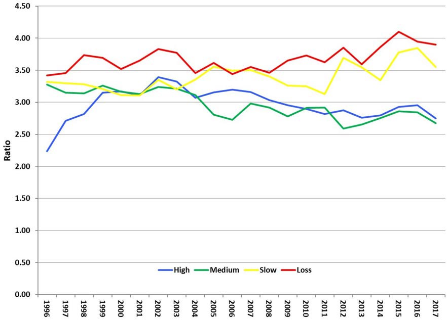
Figure 3. General fund tax revenues + fees and charges per hundreds of dollars of income.

Population-loss counties had the highest revenue effort throughout the period, and revenues per $100 of personal income increased by $.05 per $100 of income from 1996 to 2017 — the largest increase of any county type. The increase is an indicator of potential fiscal stress. In population-loss counties, in addition to increasing per capita costs, the residents who move out of the county take their incomes with them. This leaves counties with a smaller pool of resident income from which to draw revenue and pay for services. The combination of the above two factors likely explains why population-loss counties had increasing tax efforts from 1996 to 2017.

Slow-growth counties also had increasing tax effort, suggesting that county costs are increasing more rapidly than incomes. Slow-growth counties ended the period with tax effort $.02 per $100 of income higher than in 1996.

High-growth counties increased their tax efforts faster from 1996 to 2002 than any other county type. Since 2002, high-growth counties decreased their overall tax efforts. This suggests they may have reached capacity constraints early in the period, and those costs are now spread over a larger population and their fiscal stress is decreasing. Still, high-growth counties ended 2017 $.01 higher per $100 of income than in 1996

Medium-growth counties ended the period $.06 lower per $100 of income than they began. They are the only county type that decreased tax effort throughout the period, suggesting they are not experiencing fiscal stress.

General fund property and sales tax revenues as a percentage of total general fund revenues

Property and sales tax revenues tend to be 50% or more of total general fund revenues, that is, taxes are the major source of revenues for county governments. An increasing trend may be due to several factors: 1) tax bases are growing, 2) increasing tax rates, possibly because bases are not growing sufficiently to provide needed revenues or 3) other sources of revenue are declining. A decreasing trend suggests that: 1) tax bases are declining and the county is not raising tax rates, or 2) the county is generating revenue from non-tax sources, such as fees or intergovernmental revenues.

Among the county types, only slow-growth counties show a decreasing reliance on tax revenues over the entire period (Figure 4). Slow-growth counties began the period with tax revenues as a percentage of total revenues similar to those of the medium- and high-population-growth counties. Taxes were 55% of general fund revenues at the beginning of the period and ended the period at 49%. This is approximately 10 percentage points lower than every other county type. Slow-growth counties had their largest decrease in reliance on tax revenues during and immediately after the recession, 2007 to 2011.

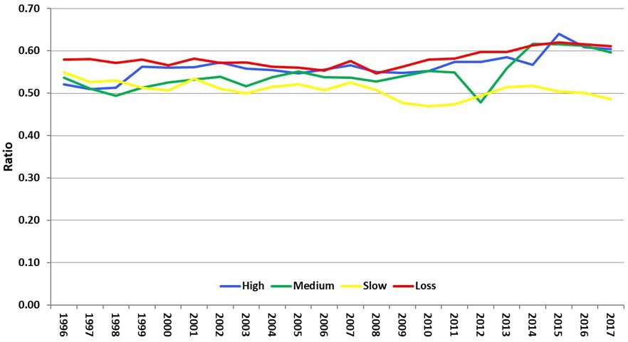
Figure 4. General fund property and sales tax revenues/General fund total revenues.

Outside factors affect budgets. For example, population-loss, medium-, and high-growth counties became increasingly reliant on property and sales taxes from 2008 to 2015, during the Great Recession and its recovery; perhaps because other revenues fell.

However, each county type had different trends in reliance on tax revenues. Population-loss counties relied on taxes more than any other county type throughout most of the period but had a small decreasing trend at the beginning, 1996 to 2008, and a slowly increasing trend from that point on. For high-growth counties, most of the increase in reliance on tax revenues is near the beginning and end of the period with a relatively stable or slightly declining ratio from 1999 to 2010. Reliance on tax revenues by medium-growth counties fluctuates throughout the period, but there is an overall trend of increasing reliance on tax revenues.

General fund property tax revenues as a percentage of total general fund tax revenues

Figure 4 shows the reliance on tax revenues in the general fund. The mix of taxes is also important. Property tax revenues as a percentage of total tax revenues shows how much counties rely on relatively stable property taxes versus the more volatile sales taxes. Property tax revenues are less than 35% of tax revenues in any county type. This means sales taxes are the largest source of tax revenue for all county types. A high reliance on sales taxes may leave a county more vulnerable to fiscal stress during economic downturns because taxable sales are more responsive to outside economic trends than are property values.

The overwhelming percentage of tax revenues are from property and sales taxes. Figure 5 demonstrates that property taxes over the period, and depending on the county type were approximately 15% to 35% of tax revenues. That means that sales taxes were approximately 85% to 65% of tax revenues. Taxable sales are a more volatile source of revenues and a higher reliance on sales taxes may lead to fiscal stress due to volatility.

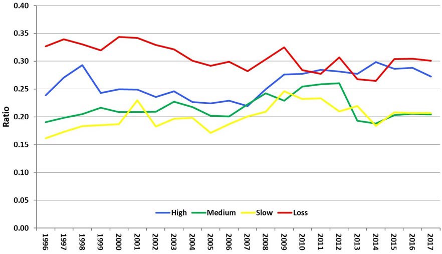
Figure 5. General fund property tax revenues/General fund total tax revenues.

Population-loss counties have the highest property tax revenues as a percentage of total tax revenues throughout most of the period. During the recession, 2007 to 2009, population-loss counties increased their reliance on property taxes, perhaps due to a drop in taxable sales. Since the recession, reliance on property tax revenues has fluctuated. However, the overall declining trend, beginning the period at 33% and ending at 30%, means there is an increasing reliance on the sales tax. Their overall declining trend in property taxes as a percentage of total tax revenues may leave population-loss counties more susceptible to fiscal stress in the event of another economic downturn.

High-, medium- and slow-growth counties all ended the period with higher reliance on property taxes than when the period began, and often had comparable trends throughout. The increase in reliance on property taxes by all county types during the recession is likely due to a decrease in taxable sales and total sales tax revenues during this period. After the recession, however, slow- and medium-growth counties decreased their reliance on property taxes but still ended the period slightly higher than in 1996. High-growth counties had the second highest reliance on property tax revenues throughout most of the period. After the recession, high-growth counties increased their reliance on property taxes.

Without asking, it is not clear why counties choose to rely on one tax base over another. In general, property taxes are not popular (Alm and Skidmore, 1999), perhaps because it is easier to see the full tax paid. Sales taxes are paid in small amounts every day, and people do not add up the total they pay, even though most people pay more each year in sales taxes than property taxes.

Fees and charges and miscellaneous revenues as a percentage of total general fund revenues

In addition to taxes and intergovernmental revenues, fees and charges and miscellaneous revenues are major components of budgets. Counties may increase fees and charges as an alternative to raising taxes. Use of these revenue sources may be easier in counties with more businesses that pay fees or that offer more services to residents and non-residents for a fee.   

Figure 6 shows the reverse of taxes as a percentage of the general fund revenues (Figure 4). The county types that rely more on taxes rely less on fees and charges and miscellaneous revenues. For population-loss, medium- and high-growth counties, fees and charges and miscellaneous revenues as a proportion of the general fund decreased from 28%–29% in 2003 and 2004 to 20% by 2017.

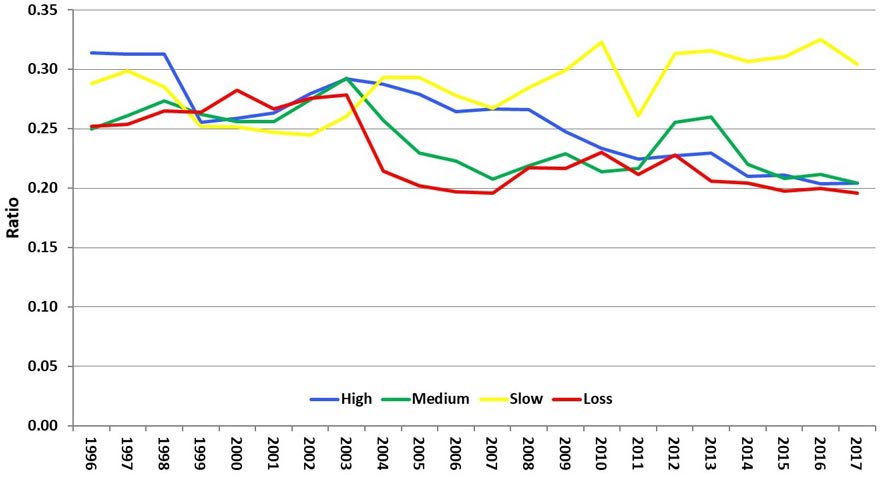
Figure 6. General fund fees and charges + miscellaneous revenues/General fund total.

Slow-growth counties had the highest reliance on these alternative own-source revenues from 2004 to 2017 (Figure 6). Only slow-growth counties increased their reliance on these alternative revenues over the period, from 24% in 2002 to 30% in 2017. Slow-growth counties have the lowest reliance on tax revenues (Figure 4) and the lowest reliance on the property tax (Figure 5). It must be noted that the increasing ratio in slow-growth counties could be due to decisions to collect more fees or to collect fewer taxes. Alternatively, it could be related to situations over which counties have limited control, such as the economy or receiving less intergovernmental revenues. Without specifically asking we cannot know the factors that influence decisions about revenue sources.

General fund intergovernmental revenues as a percentage of general fund total revenues

The main sources of intergovernmental funds are state and federal funds allocated by a set formula or by grants, such as Community Development Block Grants (CBDG) or Homeland Security, and payments in lieu of taxes. Smaller sources are other local governments paying their shares of election costs, contracts between governments, etc.

Because the majority of these revenues are subject to the decisions of other governments and not under the control of the county, increasing intergovernmental revenues as a proportion of total receipts is viewed as a potential source of fiscal stress (Maher and Nollenberger, 2009). An increasing ratio also may indicate that general fund receipts have fallen, causing the county to become more reliant on intergovernmental funds even if it is not receiving more intergovernmental revenues.

The only clear pattern that emerges is that high-growth counties slightly decreased their reliance on intergovernmental revenues and relied on them less than the other county types through most of the period (Figure 7). An important factor is the volatility of intergovernmental revenues as
a percentage of total revenues in the remaining counties. Volatility makes predicting future revenues more difficult and increases fiscal stress. The population-loss and slow-growth counties also have smaller budgets with less flexibility to respond to the volatility. The volatility of the revenues, which are outside the control of the counties, is the reason reliance on intergovernmental revenues is an indicator of fiscal stress (Maher and Nollenberger, 2009).

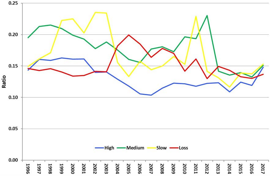
Figure 7. General intergovernmental revenues/General fund total revenues.

General fund property tax revenues as a percentage of assessed property values

General fund property tax revenues as a percentage of assessed property values reflects average county property tax rates. An increasing trend suggests the county may have insufficient revenue from other sources. Frequent changes in property tax rates also suggest that counties are having to adjust to numerous increased or unexpected expenditures. Low rates suggest that property values are high enough to generate enough revenue or that counties are relying more heavily on sales taxes and other forms of revenue. Property tax rates that are higher than other counties suggest the county might have difficulty raising rates in the future if it needs revenues (Figure 8).

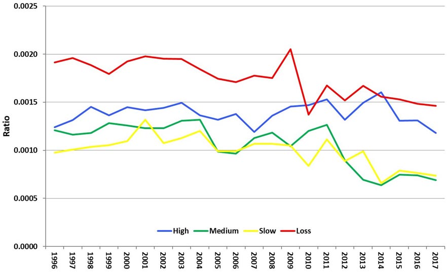
Figure 8. General fund property tax revenues/Assessed property value.

Population-loss counties have the highest property tax rates throughout most of the period, but rates decreased from 0.19% in 1996 to 0.15% in 2017. High-growth counties have the second highest property tax rates. They began and ended the period at 0.12%, but with higher rates for some years after the recession. Slow- and medium-growth counties ended the period with lower property tax rates than they began, with much of this decline occurring after the Great Recession. All county types have an overall decreasing trend leading up to the recession and increasing property tax rates during and shortly after the recession before declining again.

Assessed property value per $100s of resident income

All taxes are paid from income. Assessed property values per $100 of income shows how property values are changing relative to resident income. A decreasing trend suggests that incomes are growing more rapidly than property values. It must be noted that out-of-county property owners pay this tax, but their incomes are not included. The trends are relatively stable with the population-loss counties having the highest ratio of property values to income (Figure 9). Assessed property values per $100 of income decreased over this period in population-loss and slow-growth counties, with a small increase at the end of the period. This suggests that, in general, incomes grew more rapidly than property values. Many of the population-loss and slow-growth counties in Missouri are agricultural. Agricultural land is assessed at use value, which changes slowly. With a strong agricultural economy during much of the period, it is likely that incomes grew more rapidly than assessed values.

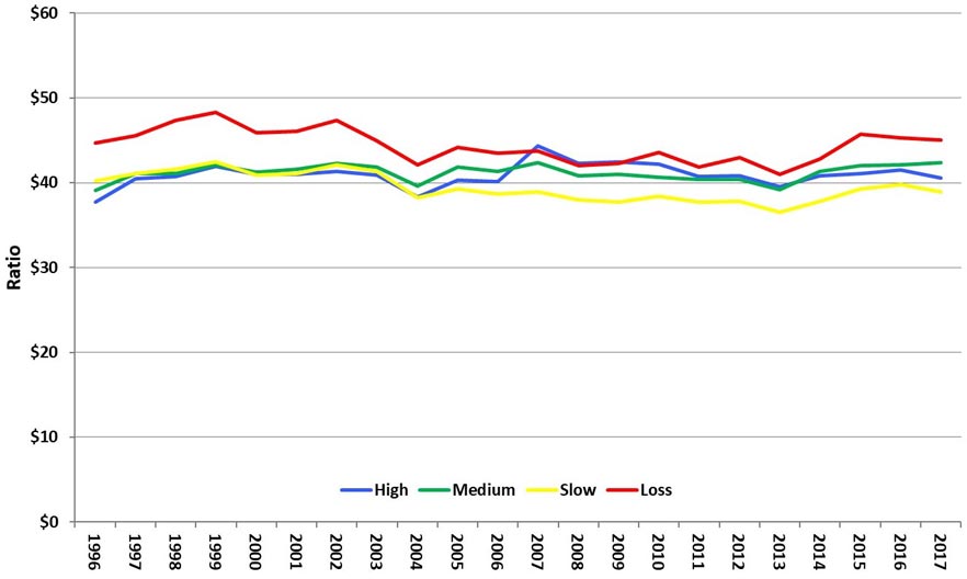
Figure 9. Assessed property value per one hundred dollars of income.

General fund sales tax revenues as a percentage of taxable sales

General fund sales tax revenues as a percentage of taxable sales shows how much the county taxes sales (Figure 10). A higher ratio indicates a higher tax rate and an increasing ratio may be an indicator of current fiscal stress. A county may face future fiscal stress if taxable sales decrease and rates are already higher than other counties.

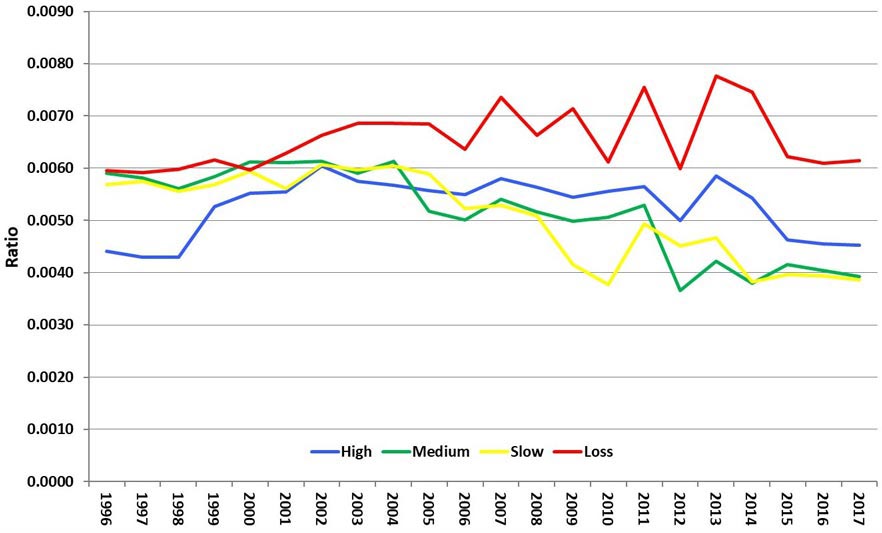
Figure 10. General fund sales tax revenues/Taxable sales.

Population-loss counties have the highest general fund sales tax revenues as a percentage of taxable sales throughout most of the period, suggesting a higher tax rate. This may be due to low taxable sales in these counties and their need to maintain revenues. Population-loss and high-growth counties ended the period with higher general fund sales tax revenues as a percentage of taxable sales, but both had declining trends after 2013. Population-loss counties show volatility beginning in the mid-2000s. Slow- and medium-growth counties had overall declining trends throughout most of the period with volatility during and after the recession.

Taxable sales per $100s of resident income

Like assessed property values per $100 of income, taxable sales per $100 of income shows how taxable sales are changing relative to resident income (Figure 11). Counties with large retail sectors will generally have higher taxable sales per $100 of income because of non-residents making purchases in those counties, and non-residents’ incomes are not included in the ratio. Population-loss counties have about $3 less taxable sales per $100 of resident income throughout the entire period than the other county types. This is likely because these counties tend to have small retail sectors even though they have higher per capita incomes.

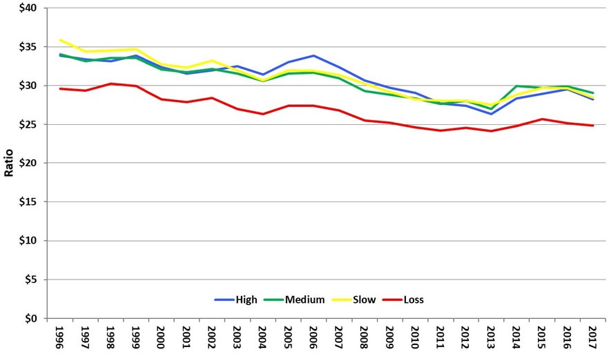
Figure 11. Taxable sales per one hundred dollars of income.

All county types during this period had decreasing taxable sales per $100 of income with the most rapid decline during the Great Recession and the recovery. These trends are likely due to short-term increased consumer and business frugality during and after the recession. In addition, there are long-run business and consumer trends of more online purchasing, some of which is not taxed by the counties, and spending more on services, most of which are not taxed in Missouri.

Cash balances as a percentage of general fund total expenditures

A measure of short-term liquidity and the ability of the county to respond to emergencies is the proportion of general funds that remain at the end of the fiscal year to expenditures for that year. It is recommended that governments carry over sufficient funds to meet a minimum of two months of expenditures because revenues are received at differing intervals during the year and there may be unanticipated expenditures or lower revenues. This translates to an ending cash balance of approximately 15% of expenditures. Given that 15% is the minimum recommendation, carrying a higher percentage may be good practice, especially for governments with small budgets (Gauthier, 2009). Overall, Figure 12 indicates that counties are following this budgeting guideline. A long-term declining trend for any county category indicates increasing fiscal stress for most counties in that population category.

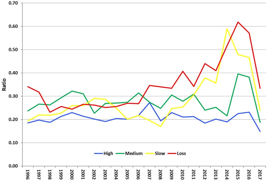
Figure 12. Cash balances/general fund total expenditures.

Several factors influence this percentage, some are government management decisions and others are outside the control of the decision makers. Revenues are influenced by revenues from other governments (mainly the state and federal), changes in tax bases, and county government management decisions. Changes in tax bases are often due to outside economic forces. Management decisions include the mix of taxes and charges and fees and the rates set for each. Intergovernmental revenues are the result of decisions by other governments as well as management decisions to apply for grants and enter into contracts. Other revenues that are management decisions include business licenses, insurance settlements, and boarding of prisoners. Expenditures also are management decisions, but include unanticipated expenditures and ones mandated by the state.

For an individual county, a declining cash balance as a percentage of total expenditures for a short period may indicate the county was saving for an expenditure and made that expenditure, or faced an unexpected expenditure. Because the data are presented as averages of types of counties, this type of short-run change for an individual county is not reflected in the trend line. All county types project declining general fund cash balances as a percentage of expenditures for the years 2016 and 2017, perhaps the result of conservative revenue projections.

Cash balances below the recommended 15%, or a trend of declining cash balances, may indicate fiscal stress. High-growth counties had both the most stable and lowest cash balances as a percentage of general fund expenditures throughout most of the period, varying between 18% and 27%. This is still above the recommended 15% minimum. High-growth counties have larger budgets, which tend to have more flexibility in them because their revenues and expenditures tend to be more diversified (Gauthier, 2009). This means these counties can more easily handle unforeseen expenditures and may not need to maintain as high a cash balance to total expenditures ratio as other county types.

Since the beginning of the Great Recession, population-loss and slow-growth counties have increased their cash balances. Slow-growth counties doubled their balances since the recession. The ratio for medium-growth counties varied between 23% and 31% from 1996 to 2014. By the end of the period, population-loss, slow-growth and medium-growth counties increased their cash balances as a percentage of total expenditures well above the recommended minimum. These increases may be a response to tightening fiscal conditions during the recession and anticipation of unforeseen expenses in the future. Their increase in short-term liquidity suggests that these county types still have the ability to respond to fiscal stress but also suggests they expect fiscal stress in the future.

General fund revenues as a percentage of all fund revenues

County budgets include the general fund, as well as the road and bridge fund, and special sales tax funds for dedicated purposes. General fund revenues as a percentage of total revenues from all funds shows how much counties rely on special funds. The higher the ratio, the less counties rely on special funds (Figure 13). The road and bridge fund is mainly supported through property taxes, while all other special funds are overwhelmingly supported with sales taxes. A high reliance on special funds, which are dedicated for specific purposes, means that counties have less flexibility to adjust to a changing economy as revenues cannot be transferred from a special fund to another fund. Smaller counties may have small sales tax bases so that they have limited ability to use special sales tax funds to support activities. That is, their budgets overall are less flexible.

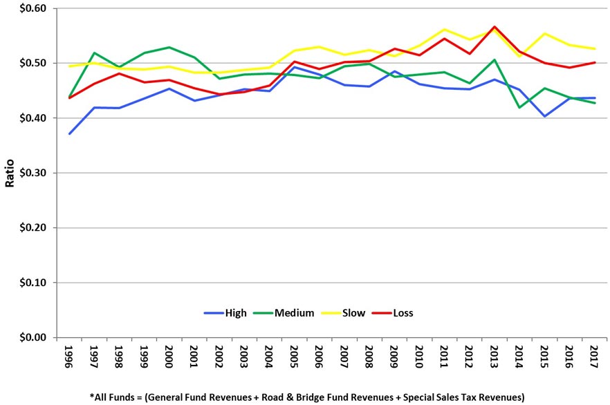
Figure 13. General fund revenues/Revenues from all funds.*

Medium-growth counties are the only county type that ended the period with a lower share of general fund revenues to all fund revenues. Their budgets may be becoming less flexible. Population-loss and slow-growth counties ended the period with 7% and 10% higher general fund revenues as a share of total revenues, and both have had higher shares than medium- and high-growth counties since the early to mid-2000s. Counties that are losing population or growing slowly may have declining taxable sales, making special sales taxes less feasible.

Summary

Local governments need a way to evaluate their budget fiscal condition over time in order to pinpoint the sources of budget stress — are they short run, such as the recession or a natural disaster, or are they part of longer-term trends? Businesses monitor their financial condition using a set of financial ratios. A similar approach can be useful for governments. The set of fiscal ratios used in this report focuses on the short run because it does not include debt. No single ratio can reflect the complexity of local government budgets. The set of fiscal ratios in the report is calculated from the budgets of Missouri’s third class counties.

The focus of this paper is on long-term trends in population that can affect the fiscal condition of counties. Population change can have a major impact on county budgets because it can affect whether per capita, or per citizen, costs of providing public services are increasing or decreasing. For example, population loss increases per capita costs, requiring a greater tax effort to maintain services and putting stress on the budget. High-population-growth counties must periodically address capacity constraints, which may result in periodic per capita cost increases that can be exacerbated by economic shifts. An understanding of how population change affects county fiscal condition can help county governments adopt policies to make county finances more resilient to fiscal stress.

Differing economic factors between counties may alleviate or magnify the effects of population loss. For example, population-loss counties in the agricultural area in northern Missouri may have benefited from a strong agricultural economy during much of the period examined, making local budgets more stable. Non-agricultural population-loss counties in southern Missouri may have experienced greater budget stresses.

Population-loss counties rely more on taxes than the other counties. Slow-population-growth counties rely more on fees, charges and miscellaneous revenues. Because these revenues are likely influenced by short-run economic factors, these counties may face more budget instability. All counties rely more on sales tax revenues than on property tax revenues. Taxable sales are a less stable tax base than are assessed property values, making county budgets more subject to short-run economic trends and more volatility.

Reliance on special funds, the revenues of which are dedicated to a specific purpose, reduces flexibility in budgeting. The population-loss and slow-growth counties are increasing their reliance on the general fund, providing budget flexibility. The moderate-growth counties are increasing their reliance on special funds. Since the recession, the high-growth counties also have increased their reliance on special funds. In Missouri, most of the special funds are funded by sales taxes. Counties that are increasing their reliance on special funds are also increasing their reliance on the less stable sales tax base.

Intergovernmental revenues are a volatile source of revenues, which contributes to budget stresses in all counties. In general, the counties are following good management practices of having an ending cash balance of 15% or more.

References

• Aldag, Austin M. and Mildred E. Warner, and Yunji Kim. (2017). “What Causes Local fiscal Stress? What Can Be Done About It?” Department of City and Regional Planning, Cornell University Ithaca, NY. https://labs.aap.cornell.edu/sites/aap-labs/files/2022-09/Aldag%20et.al_2017a.pdf
• Alm, James and Mark Skidmore. (1999). “Why Do Tax and Expenditure Limitations Pass in State Elections?” Public Finance Review. 27(5):481–510
• Bel, German and Mildred E. Warner. (2015). “Inter-Municipal Cooperation and Costs: Expectations and Evidence.” Public Administration. 93(1): 52–67.
• Brown, K.W. (1993). “The 10-Point Test of Financial Condition: Toward an Easy-to-Use Assessment Tool for Smaller Cities. Government Finance Review. 9(6):21–26
• Department of Revenue (2017). “Local Government Tax Guide.” https://dor.mo.gov/forms/4890.pdf
• Economic Research Service (ERS) (2017). “County Economic Types, 2015 Edition.” United States Department of Agriculture. https://www.ers.usda.gov/data-products/county-typology-codes/descriptions-and-maps.aspx#farming
• Gauthier, Stephen J. (2009). “GFOA Updates Best Practice on Fund Balance.” Government Finance Review. 25(6): 68–69.
• Kevin-Myers, Bridget and Russ Hembree, 2012. “The Hancock Amendment: Missouri’s Tax Limitation Measure.” Missouri Legislative Academy. Institute of Public Policy, University of Missouri. https://mospace.umsystem.edu/xmlui/handle/10355/2888
• Maher, Craig S. and Karl Nollenberger. (2009). “Revisiting Kenneth Brown’s “10-Point Test.” Government Finance Review. 25(5): 61-66.
• Penton Media Inc. (2018). “Municipal Cost Index.” American City & County. http://americancityandcounty.com/mciarchive
• Stallmann, Judith I. and Thomas G. Johnson. “Thinking of Tax Policy as a Portfolio.” Institute of Public Policy, Missouri Legislative Academy, Report 14-2011. Harry S Truman School of Public Affairs. October 2011. https://www.researchgate.net/publication/272790370_Thinking_of_Tax_Policy_as_a_Portfolio